Bootstrapping and Confidence Intervals

Answers for Question 3 in Quiz 12

Load Libraries

library(tidyverse)
library(infer)
library(fivethirtyeight)
library(dplyr)
library(ggplot2)
library(here)

Look at the Variable Definitions in congress_age

• What is the average age of members that have served in congress?
• Set random seed generator to 123
• Take a sample of 100 from the dataset congress_age and assign it to congress_age_100

set.seed(123)
congress_age_100 <- congress_age %>% 
  rep_sample_n(size = 100)
show(congress_age)

# A tibble: 18,635 x 13
   congress chamber bioguide firstname middlename lastname  suffix
      <int> <chr>   <chr>    <chr>     <chr>      <chr>     <chr> 
 1       80 house   M000112  Joseph    Jefferson  Mansfield <NA>  
 2       80 house   D000448  Robert    Lee        Doughton  <NA>  
 3       80 house   S000001  Adolph    Joachim    Sabath    <NA>  
 4       80 house   E000023  Charles   Aubrey     Eaton     <NA>  
 5       80 house   L000296  William   <NA>       Lewis     <NA>  
 6       80 house   G000017  James     A.         Gallagher <NA>  
 7       80 house   W000265  Richard   Joseph     Welch     <NA>  
 8       80 house   B000565  Sol       <NA>       Bloom     <NA>  
 9       80 house   H000943  Merlin    <NA>       Hull      <NA>  
10       80 house   G000169  Charles   Laceille   Gifford   <NA>  
# ... with 18,625 more rows, and 6 more variables: birthday <date>,
#   state <chr>, party <chr>, incumbent <lgl>, termstart <date>,
#   age <dbl>

1

Use specify to indicate the variable from congress_age_100 that you are interested in

congress_age_100 %>% 
  specify(response = age)

Response: age (numeric)
# A tibble: 100 x 1
     age
   <dbl>
 1  53.1
 2  54.9
 3  65.3
 4  60.1
 5  43.8
 6  57.9
 7  55.3
 8  46  
 9  42.1
10  37  
# ... with 90 more rows

2

generate 1000 replicates of your sample of 100

congress_age_100  %>% 
  specify(response = age)  %>% 
  generate(reps = 1000, type= "bootstrap")

Response: age (numeric)
# A tibble: 100,000 x 2
# Groups:   replicate [1,000]
   replicate   age
       <int> <dbl>
 1         1  42.1
 2         1  71.2
 3         1  45.6
 4         1  39.6
 5         1  56.8
 6         1  71.6
 7         1  60.5
 8         1  56.4
 9         1  43.3
10         1  53.1
# ... with 99,990 more rows

3

• Assign to bootstrap_distribution_mean_age
• Display bootstrap_distribution_mean_age

bootstrap_distribution_mean_age  <- congress_age_100  %>% 
  specify(response = age)  %>% 
  generate(reps = 1000, type = "bootstrap")  %>% 
  calculate(stat = "mean")

bootstrap_distribution_mean_age

# A tibble: 1,000 x 2
   replicate  stat
       <int> <dbl>
 1         1  53.6
 2         2  53.2
 3         3  52.8
 4         4  51.5
 5         5  53.0
 6         6  54.2
 7         7  52.0
 8         8  52.8
 9         9  53.8
10        10  52.4
# ... with 990 more rows

4

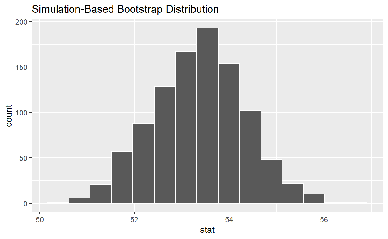
visualize the bootstrap distribution

visualise(bootstrap_distribution_mean_age)

Calculate the 95% confidence interval using the percentile method

• Assign the output to congress_ci_percentile
• Display congress_ci_percentile

congress_ci_percentile  <- bootstrap_distribution_mean_age %>% 
  get_confidence_interval(type = "percentile", level = 0.95)

congress_ci_percentile

# A tibble: 1 x 2
  lower_ci upper_ci
     <dbl>    <dbl>
1     51.5     55.2

• Calculate the observed point estimate of the mean and assign it to obs_mean_age
• Display obs_mean_age

obs_mean_age <- congress_age_100 %>% 
  specify(response = age) %>% 
  calculate(stat = "mean") %>% 
  pull()

obs_mean_age

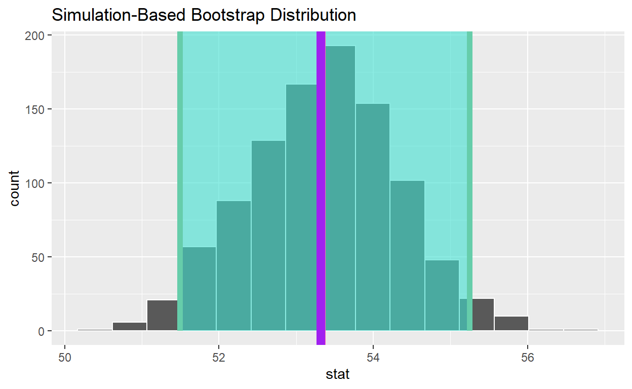
[1] 53.36

• Shade the confidence interval
• Add a line at the observed mean, obs_mean_age, to your visualization and color it “hotpink”

visualize(bootstrap_distribution_mean_age) +
  shade_confidence_interval(endpoints = congress_ci_percentile) +
  geom_vline(xintercept = obs_mean_age, color = "hotpink", size = 1)

• Calculate the population mean to see if it is in the 95% confidence interval
• Assign the output to pop_mean_age
• Display pop_mean_age

pop_mean_age <- congress_age %>% 
  summarise(pop_mean = mean(age)) %>% 
  pull()

pop_mean_age

[1] 53.31373

Add a line to the visualiztin at the, population mean, pop_mean_age, to the plot color it “purple”

visualize(bootstrap_distribution_mean_age) +
  shade_confidence_interval(endpoints = congress_ci_percentile) + 
  geom_vline(xintercept = obs_mean_age, color = "hotpink", size = 1) +
  geom_vline(xintercept = pop_mean_age, color = "purple", size = 3) 

Change set.seed(123) to set.seed(4346). Rerun all the code.

Look at the Variable Definitions in congress_age

• What is the average age of members that have served in congress?
• Set random seed generator to 123
• Take a sample of 100 from the dataset congress_age and assign it to congress_age_100

set.seed(4346)
congress_age_100 <- congress_age %>% 
  rep_sample_n(size = 100)
show(congress_age)

# A tibble: 18,635 x 13
   congress chamber bioguide firstname middlename lastname  suffix
      <int> <chr>   <chr>    <chr>     <chr>      <chr>     <chr> 
 1       80 house   M000112  Joseph    Jefferson  Mansfield <NA>  
 2       80 house   D000448  Robert    Lee        Doughton  <NA>  
 3       80 house   S000001  Adolph    Joachim    Sabath    <NA>  
 4       80 house   E000023  Charles   Aubrey     Eaton     <NA>  
 5       80 house   L000296  William   <NA>       Lewis     <NA>  
 6       80 house   G000017  James     A.         Gallagher <NA>  
 7       80 house   W000265  Richard   Joseph     Welch     <NA>  
 8       80 house   B000565  Sol       <NA>       Bloom     <NA>  
 9       80 house   H000943  Merlin    <NA>       Hull      <NA>  
10       80 house   G000169  Charles   Laceille   Gifford   <NA>  
# ... with 18,625 more rows, and 6 more variables: birthday <date>,
#   state <chr>, party <chr>, incumbent <lgl>, termstart <date>,
#   age <dbl>

1 Use specify to indicate the variable from congress_age_100 that you are interested in

congress_age_100 %>% 
  specify(response = age)

Response: age (numeric)
# A tibble: 100 x 1
     age
   <dbl>
 1  58  
 2  27.3
 3  59.4
 4  47.8
 5  36.4
 6  62.3
 7  52.5
 8  55.5
 9  44  
10  48  
# ... with 90 more rows

2 generate 1000 replicates of your sample of 100

congress_age_100  %>% 
  specify(response = age)  %>% 
  generate(reps = 1000, type= "bootstrap")

Response: age (numeric)
# A tibble: 100,000 x 2
# Groups:   replicate [1,000]
   replicate   age
       <int> <dbl>
 1         1  55.2
 2         1  40.8
 3         1  55.7
 4         1  52.5
 5         1  54.5
 6         1  35.8
 7         1  44.5
 8         1  47.9
 9         1  40.8
10         1  37.4
# ... with 99,990 more rows

3 - Assign to bootstrap_distribution_mean_age - Display bootstrap_distribution_mean_age

bootstrap_distribution_mean_age  <- congress_age_100  %>% 
  specify(response = age)  %>% 
  generate(reps = 1000, type = "bootstrap")  %>% 
  calculate(stat = "mean")

bootstrap_distribution_mean_age

# A tibble: 1,000 x 2
   replicate  stat
       <int> <dbl>
 1         1  51.3
 2         2  48.2
 3         3  49.7
 4         4  50.5
 5         5  51.6
 6         6  47.9
 7         7  49.5
 8         8  50.0
 9         9  51.0
10        10  51.0
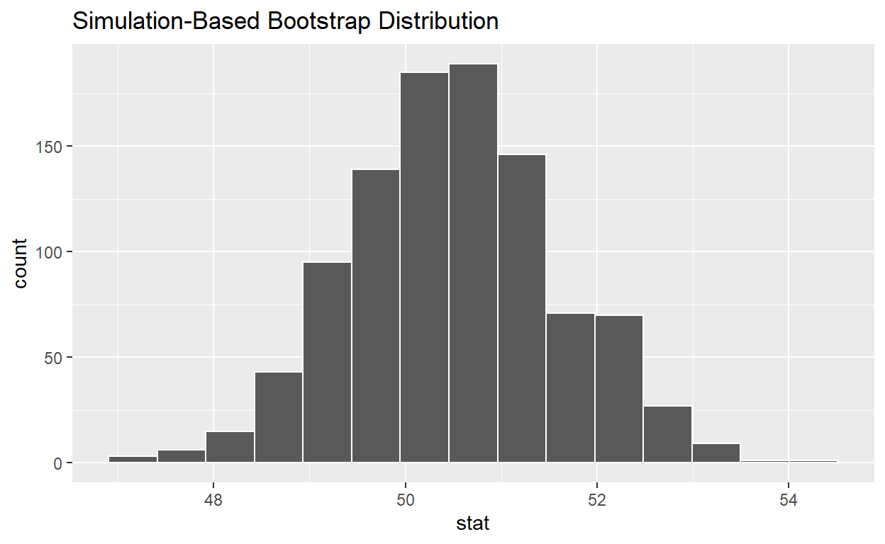
# ... with 990 more rows

4 visualize the bootstrap distribution

visualise(bootstrap_distribution_mean_age)

Calculate the 95% confidence interval using the percentile method

• Assign the output to congress_ci_percentile
• Display congress_ci_percentile

congress_ci_percentile  <- bootstrap_distribution_mean_age %>% 
  get_confidence_interval(type = "percentile", level = 0.95)

congress_ci_percentile

# A tibble: 1 x 2
  lower_ci upper_ci
     <dbl>    <dbl>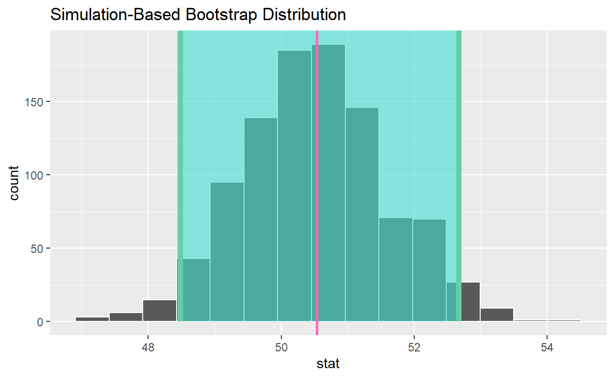
1     48.5     52.7

• Calculate the observed point estimate of the mean and assign it to obs_mean_age
• Display obs_mean_age

obs_mean_age <- congress_age_100 %>% 
  specify(response = age) %>% 
  calculate(stat = "mean") %>% 
  pull()

obs_mean_age

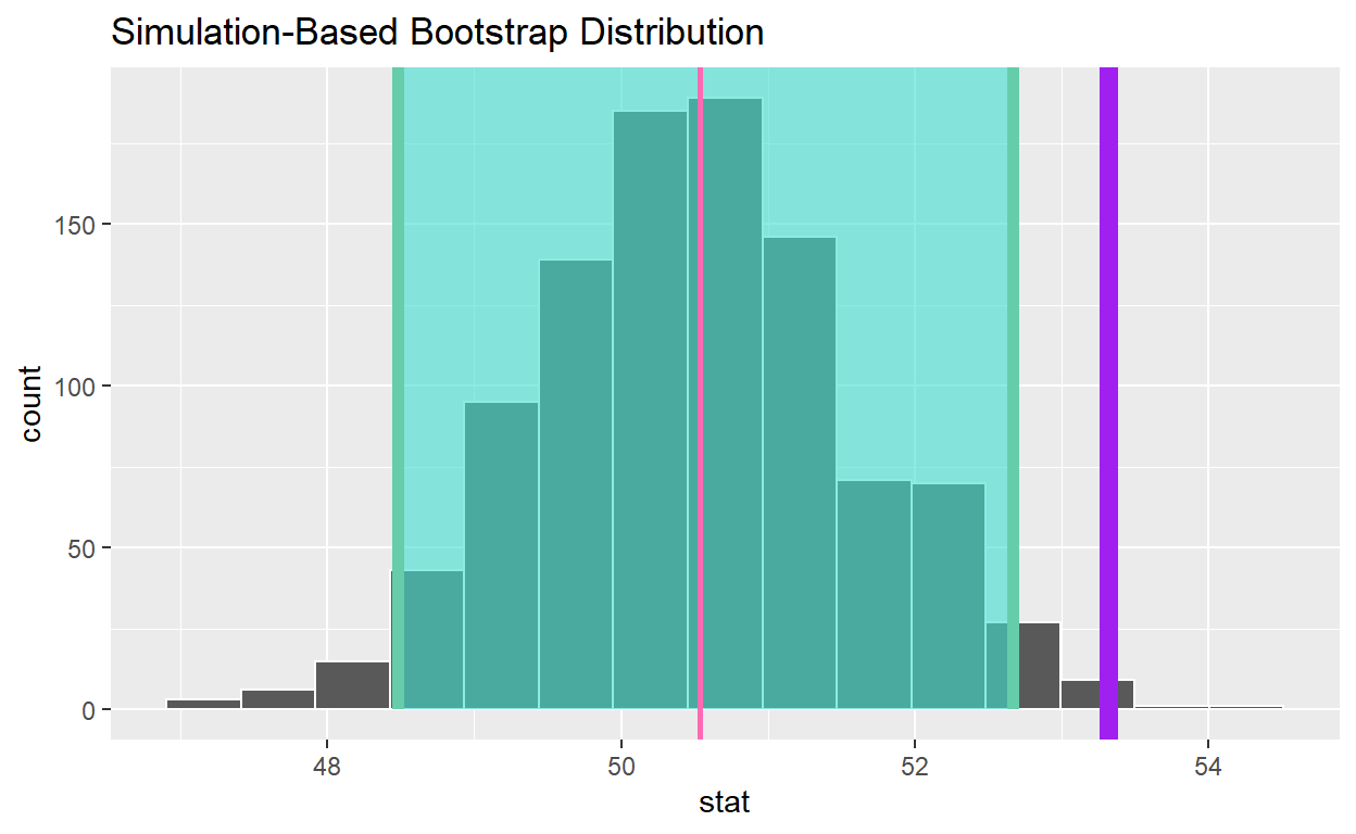
[1] 50.533

• Shade the confidence interval
• Add a line at the observed mean, obs_mean_age, to your visualization and color it “hotpink”

visualize(bootstrap_distribution_mean_age) +
  shade_confidence_interval(endpoints = congress_ci_percentile) +
  geom_vline(xintercept = obs_mean_age, color = "hotpink", size = 1)

• Calculate the population mean to see if it is in the 95% confidence interval
• Assign the output to pop_mean_age
• Display pop_mean_age

pop_mean_age <- congress_age %>% 
  summarise(pop_mean = mean(age)) %>% 
  pull()

pop_mean_age

[1] 53.31373

Add a line to the visualiztin at the, population mean, pop_mean_age, to the plot color it “purple”

visualize(bootstrap_distribution_mean_age) +
  shade_confidence_interval(endpoints = congress_ci_percentile) + 
  geom_vline(xintercept = obs_mean_age, color = "hotpink", size = 1) +
  geom_vline(xintercept = pop_mean_age, color = "purple", size = 3) 

ggsave("pop_mean_age_plot.png", 
       path = here("_posts", "2021-05-11-bootsrtapping-and-confidence-intervals"))