My Blog: Sampling

Load Libraries

library(tidyverse)
library(moderndive)
library(ggplot2)
library(here)

1.a

Take 1180 samples of size of 26 instead of 1000 replicates of size 25 from the bowl dataset. Assign the output to virtual_samples_26

virtual_samples_26 <- bowl %>% 
  rep_sample_n(size = 26, reps = 1180)

1.b

Compute resulting 1180 replicates of proportion red

start with virtual_samples_26 THEN
group_by replicate THEN
create variable red equal to the sum of all the red balls
create variable prop_red equal to variable red / 26
Assign the output to virtual_prop_red_26

virtual_prop_red_26 <- virtual_samples_26 %>% 
  group_by(replicate) %>% 
  summarize(red = sum(color == "red")) %>% 
  mutate(prop_red = red / 26)

1.c

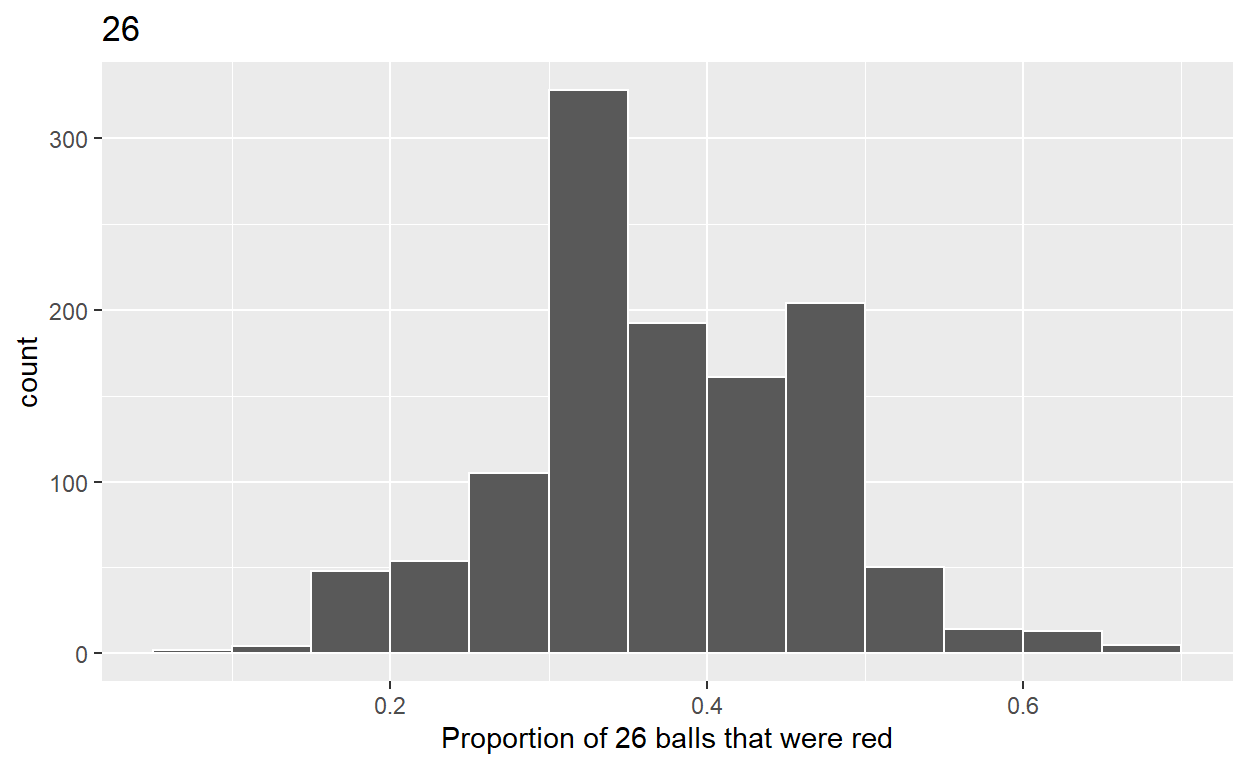
Plot distribution of virtual_prop_red_26 via a histogram use labs to

label x axis = “Proportion of 26 balls that were red”
create title = “26”

ggplot(virtual_prop_red_26, aes(x = prop_red)) +
  geom_histogram(binwidth = 0.05, boundary = 0.4, color = "white") +
  labs(x = "Proportion of 26 balls that were red", title = "26")

2.a

Take 1180 samples of size of 55 instead of 1000 replicates of size 50. Assign the output to virtual_samples_55

virtual_samples_55 <- bowl %>% 
  rep_sample_n(size = 55, reps = 1180)

2.b

Compute resulting 1180 replicates of proportion red

start with virtual_samples_55 THEN
group_by replicate THEN
create variable red equal to the sum of all the red balls
create variable prop_red equal to variable red / 55
Assign the output to virtual_prop_red_55

virtual_prop_red_55 <- virtual_samples_55 %>% 
  group_by(replicate) %>% 
  summarize(red = sum(color == "red")) %>% 
  mutate(prop_red = red / 55)

2.c

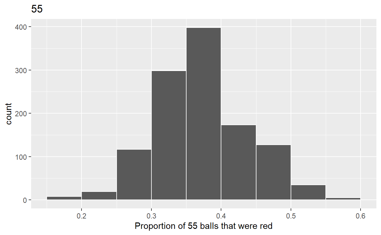
Plot distribution of virtual_prop_red_55 via a histogram use labs to

label x axis = “Proportion of 55 balls that were red”
create title = “55”

ggplot(virtual_prop_red_55, aes(x = prop_red)) +
  geom_histogram(binwidth = 0.05, boundary = 0.4, color = "white") +
  labs(x = "Proportion of 55 balls that were red", title = "55")

3.a

Take 1180 samples of size of 110 instead of 1000 replicates of size 50. Assign the output to virtual_samples_55

virtual_samples_110 <- bowl %>% 
  rep_sample_n(size = 110, reps = 1180)

3.b

Compute resulting 1180 replicates of proportion red

start with virtual_samples_55 THEN
group_by replicate THEN
create variable red equal to the sum of all the red balls
create variable prop_red equal to variable red / 55
Assign the output to virtual_prop_red_55

virtual_prop_red_110 <- virtual_samples_110 %>% 
  group_by(replicate) %>% 
  summarize(red = sum(color == "red")) %>% 
  mutate(prop_red = red / 110)

3.c

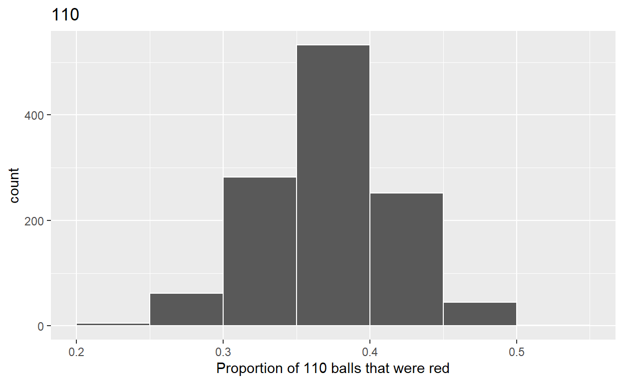
Plot distribution of virtual_prop_red_55 via a histogram use labs to

label x axis = “Proportion of 55 balls that were red”
create title = “55”

ggplot(virtual_prop_red_110, aes(x = prop_red)) +
  geom_histogram(binwidth = 0.05, boundary = 0.4, color = "white") +
  labs(x = "Proportion of 110 balls that were red", title = "110")

# save plot for post preview
ggsave("prop_of_110.png", 
       path = here("_posts", "2021-05-04-sampling"))

Standard Deviations

n = 26

virtual_prop_red_26 %>% 
  summarise(sd = sd(prop_red))

# A tibble: 1 x 1
      sd
   <dbl>
1 0.0969

n = 55

virtual_prop_red_55 %>% 
  summarise(sd = sd(prop_red))

# A tibble: 1 x 1
      sd
   <dbl>
1 0.0661

n = 110

virtual_prop_red_110 %>% 
  summarise(sd = sd(prop_red))

# A tibble: 1 x 1
      sd
   <dbl>
1 0.0448